Example Flow: Grid Smoothing

This article outlines how to use Flows to generate and smooth a grid. This uses the following building blocks:

• LogInput
• CpiLogCalc
• PointsSelect
• PointsToGrid
• GridOutput
• GridSmooth
• GridOutput

The assembled flow is shown below:

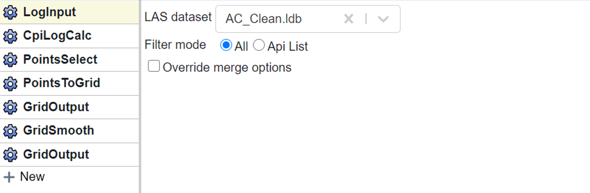
In the LogInput block select the database of interest using the dropdown menu. Use the “All” option to use all the wells in your database for performing the operation.

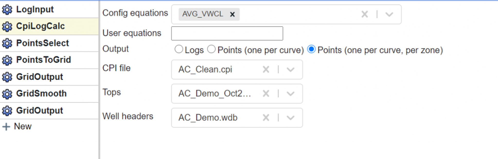
In the CpiLogCalc option we can either choose to use equations that are already available in the CPI Config (see a list of common curve names here) or use our own equation. In this example I have chosen to use the average vclay curve.

This equation calculates the average Vclay by zone in our CPI file. Finally we will select the CPI file, and tops and well headers database that we want to use. This is important because the CPI file is required to make sure that all the parameters are correctly captured.

Because we are going to generate a grid, we have the CpiLogCalc output Points. We set this at one per curve, per zone. If we were using a byStatsWindow function we would use the one per curve option.

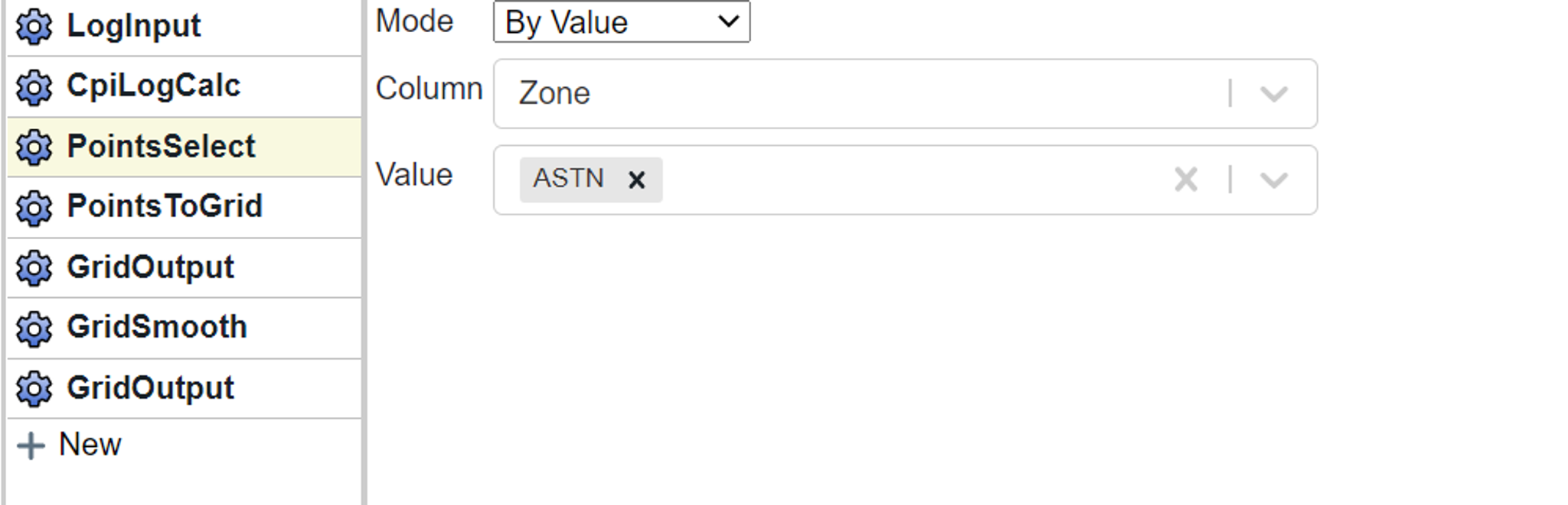
In the PointsSelect block we choose the zone that we wish to grid – in this case the Austin Chalk, abbreviated ASTN.

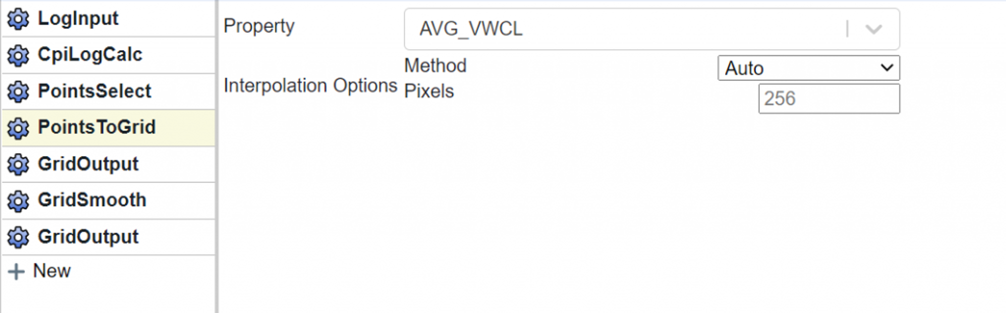
In the PointsToGrid block we select the property to grid, then choose the gridding algorithm we would like to use.

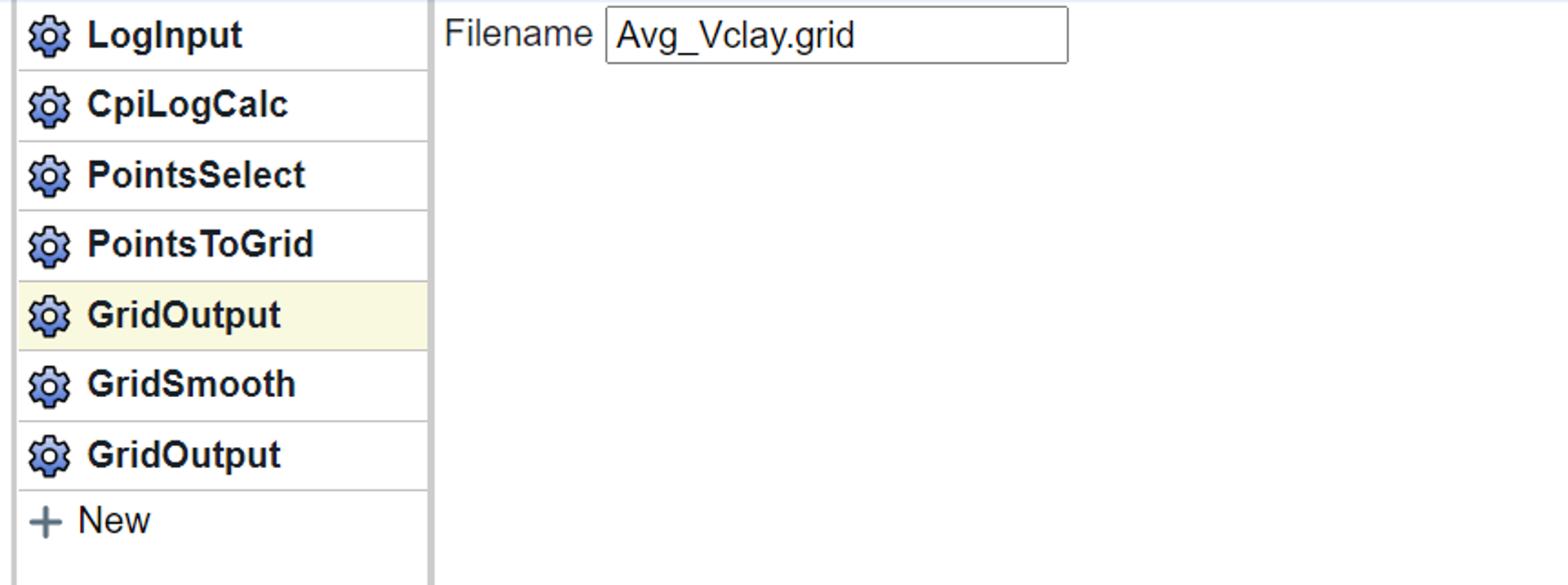
In the first GridOutput block, which is optional, we provide a name. This is not our final smoothed grid, but an unsmoothed version. We are saving it in this example so we can do a comparison of pre- and post-smoothed versions if needed.

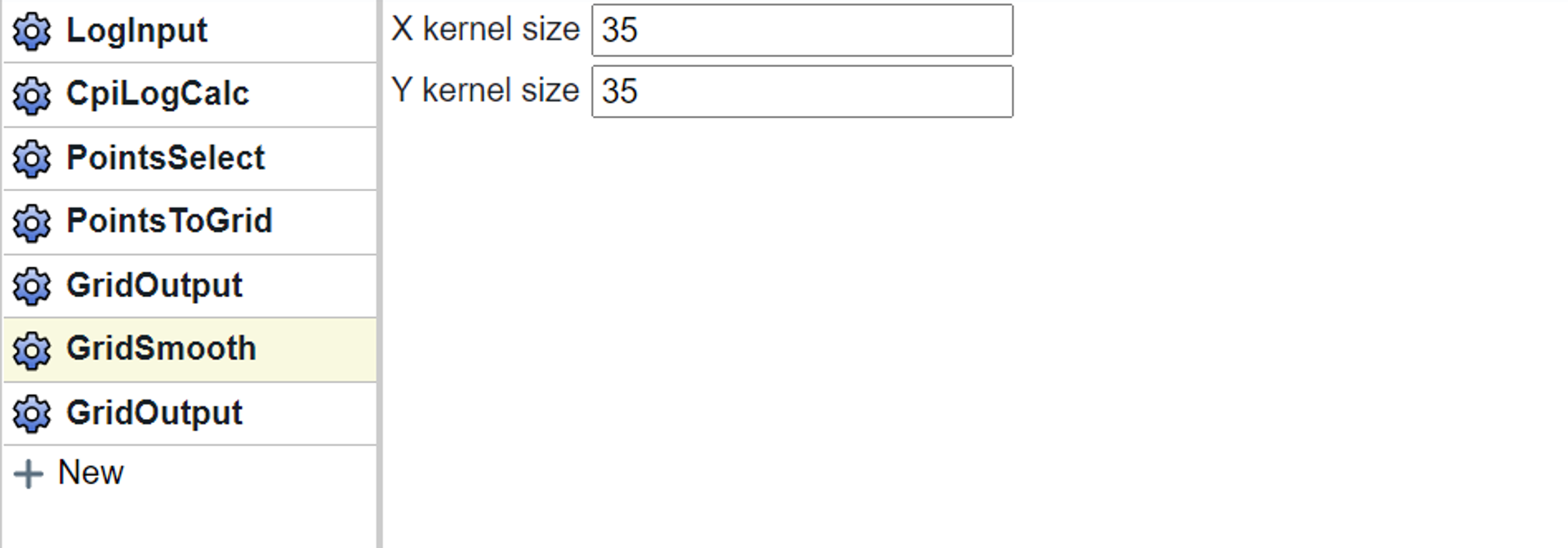
In the GridSmooth block we set a kernel size for the smoothing – larger values smooth more aggressively. In most instances you will likely want the X kernel = Y kernel, but this is not required.

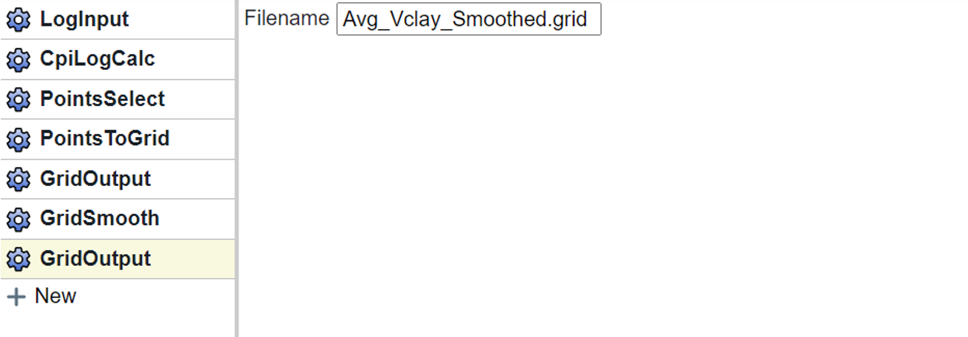
And finally we will use the second GridOutput block to write out our final smoothed map. It will be written to the folder that the Flow resides in.