Example Flow: Isopach Maps
This article outlines how to use Flows to generate isopach maps using Flows in Danomics. Although there are multiple ways to generate isopach maps in the platform, in this article we’ll do it using the TopsToIsochorePoints Flow block. The Flow tools blocks used include the following:
- PointsInput: Add tops data to the flow
- TopsToTVD: Put the tops in TVD space
- TopsToIsochorePoints: Evaluate the thickness of each zone
- PointsToGrid: Generate a grid of each zone
- GridOutput: Write the results to a multi-grid file
In this example we generate grids; however, we could write out the isochore points instead. To do this, remove the last two blocks and add a PointsOutput block in their place.
Example Flow
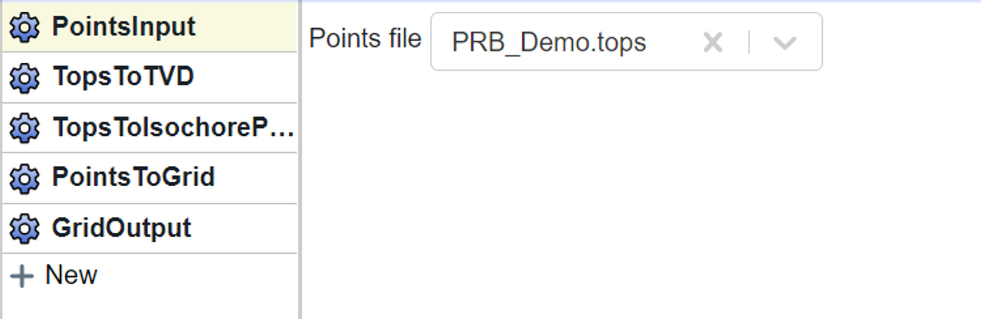
The PointsInput block is used to bring tops data into the flow.
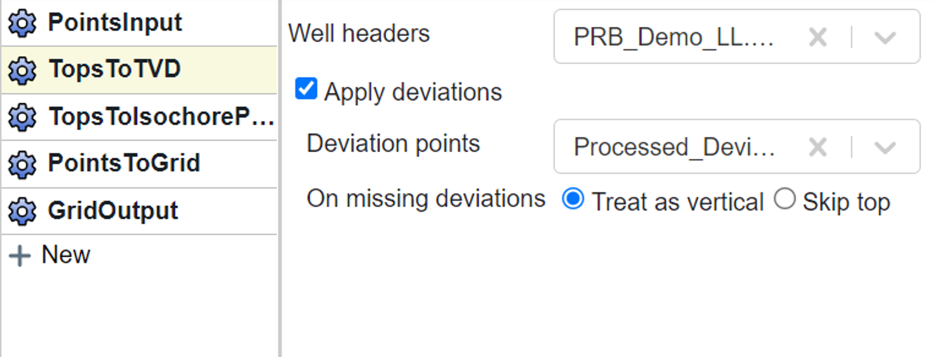
The TopsToTVD block allows us to select the well headers to use and (optionally) choose the deviation survey data.
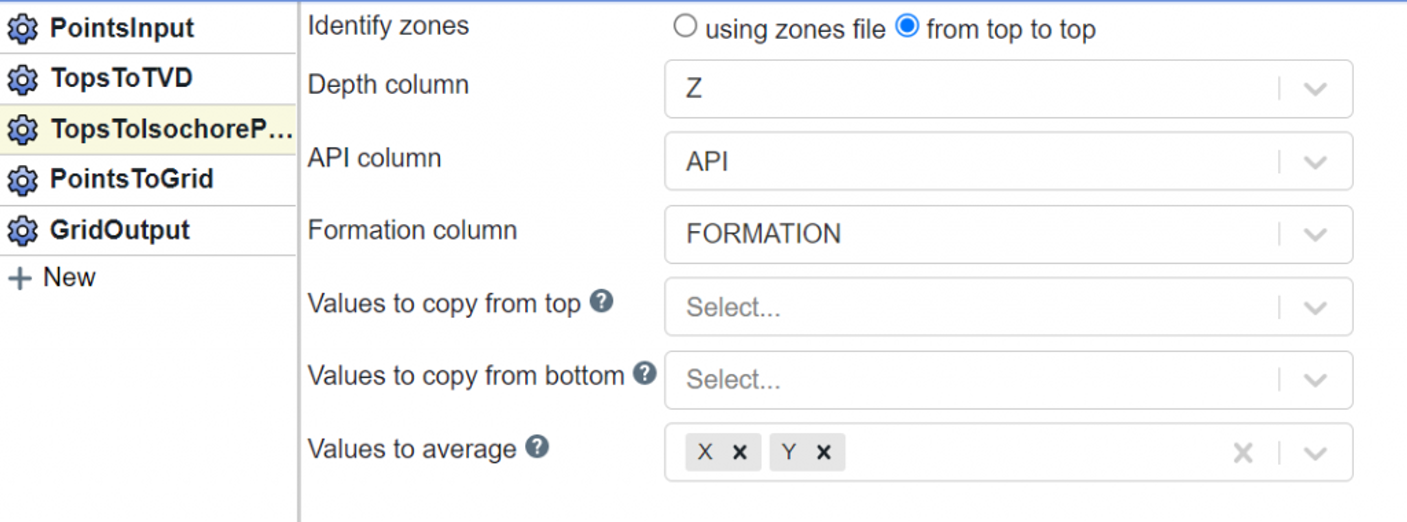
The TopsToIsochorePoints block determines the thickness of each zone. There are several important options that should be considered. The “Identify zones” option lets you select if you want to perform the calculation using either a “.zones” file or top to top. In most cases it is considered best practice to use a “.zones” file definition. This is best illustrated with an example. Let’s say the stratigraphy comprises three zones A, B, and C. If you select top to top for a well with all three zones, you will get thickness values for zone A (A to B) and zone B (B to C). However, in a well that only has tops for A and C, you will get a thickness value for zone A that comprises the entire interval from A to C – this is likely not the desired behavior. If you choose to use a zones file then you will define zone A as always being A to B and zone B as always being B to C. Therefore, in a well with all three zones you will still get the same values as you would for top to top. However, in a well with just tops A and C, you will not get a result because that well doesn’t satisfy the requirements for a valid zone A (base of zone is missing) or B (top of zone is missing).
The other major consideration is to decide where in space to map the result. “Copy from top” allows you to define the X/Y coordinates at the top of the zone. “Copy from bottom” allows you to define the X/Y coordinates at the bottom of the zone. “Values to average” let’s you average coordinates from the top and bottom of the zone. For vertical wells there will be no difference between the three options. For deviated wells the behavior is:
- Copy from top: maps value at the top of the formation
- Copy from bottom: maps value at the base of the formation
- Values to average: maps value at an average of the X/Y values at top/base of the formation.
If dealing with highly deviated wells the “Values to average” option should be used.
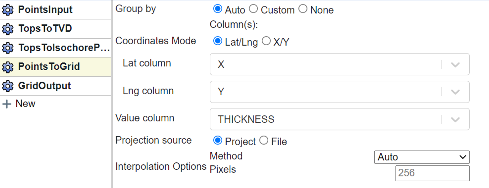
The PointsToGrid block let’s you select what property to map. In this case zone “Thickness”.
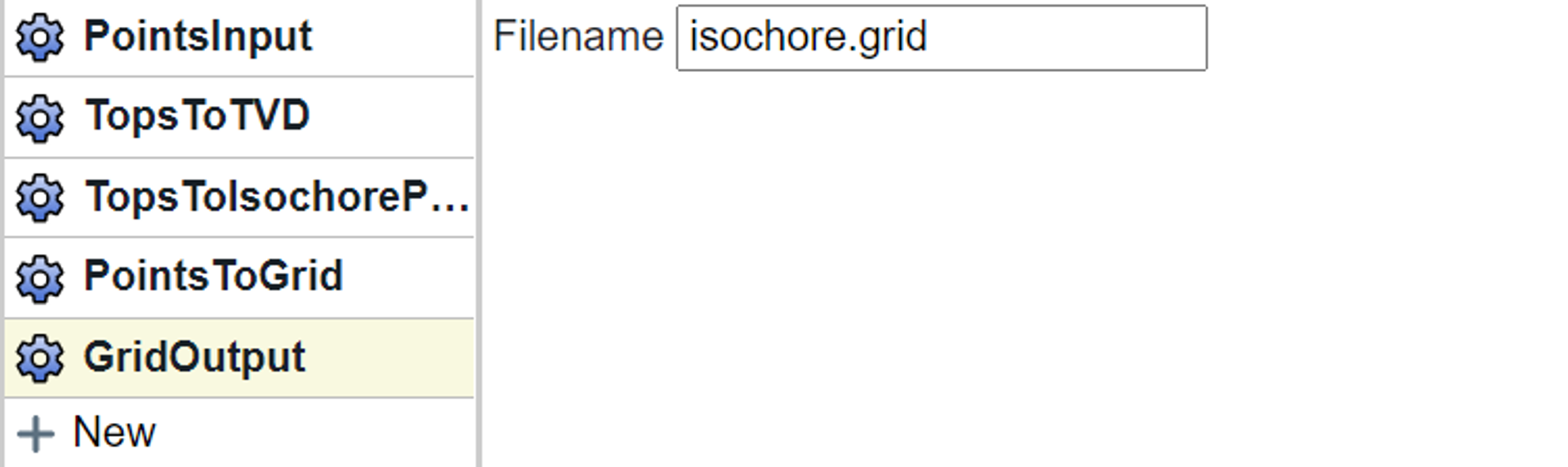
Finally, we end with a GridOutput block where you provide a name to the resulting multigrid file.
Summary
In this example flow we brought tops data into the flow, converted it to TVD space, and then generated isochore points that we were able to map. There were several options that we needed to set for the TopsToIsochorePoints block to ensure that our results matched our expectations – most important of which is defining zones.
Tags
Related Insights
DCA: Type well curves
In this video I demonstrate how to generate a well set filtered by a number of criteria and generate a multi-well type curve. Before starting this video you should already know how to load your data and create a DCA project. If not, please review those videos. Type well curves are generated by creating a decline that represents data from multiple wells.
DCA: Loading Production data
In this video I demonstrate how to load production and well header data for use in a decline curve analysis project. The first step is to gather your data. You’ll need: Production data – this can be in CSV, Excel, or IHS 298 formats. For spreadsheet formats you’ll need columns for API, Date, Oil, Gas, Water (optional), and days of production for that period (optional). Well header data – this can be in CSV, Excel, or IHS 297 formats.
Sample data to get started
Need some sample data to get started? The files below are from data made public by the Wyoming Oil and Gas Commission. These will allow you to get started with petrophysics, mapping, and decline curve analysis. Well header data Formation tops data Deviation survey data Well log data (las files) Production data (csv) or (excel) Wyoming counties shapefile and projection Wyoming townships shapefile and projection Haven’t found the help guide that you are looking for?