Fluid Substitution Modelling
In Danomics Petrophysics users are guided through a workflow that walks them through a number of modules. These modules are located via a dropdown menu at the top center of the window. The modules are listed in the order in which a user should ideally proceed through a project. However, this order is not strictly enforced and the user can start at any module and can seamlessly move both forward and back through the modules. This help article will focus on the Fluid Substitution Modelling module.
Fluid Substitution Modelling
The Fluid Substitution Modelling module is an advanced module designed to help users understand the affects of changes in hydrocarbon composition and saturation on the sonic and shear sonic logs. This module can be accessed by selecting “Fluid Substitution Modelling” from the module selection dropdown menu in the top-center of the screen.
Use Cases
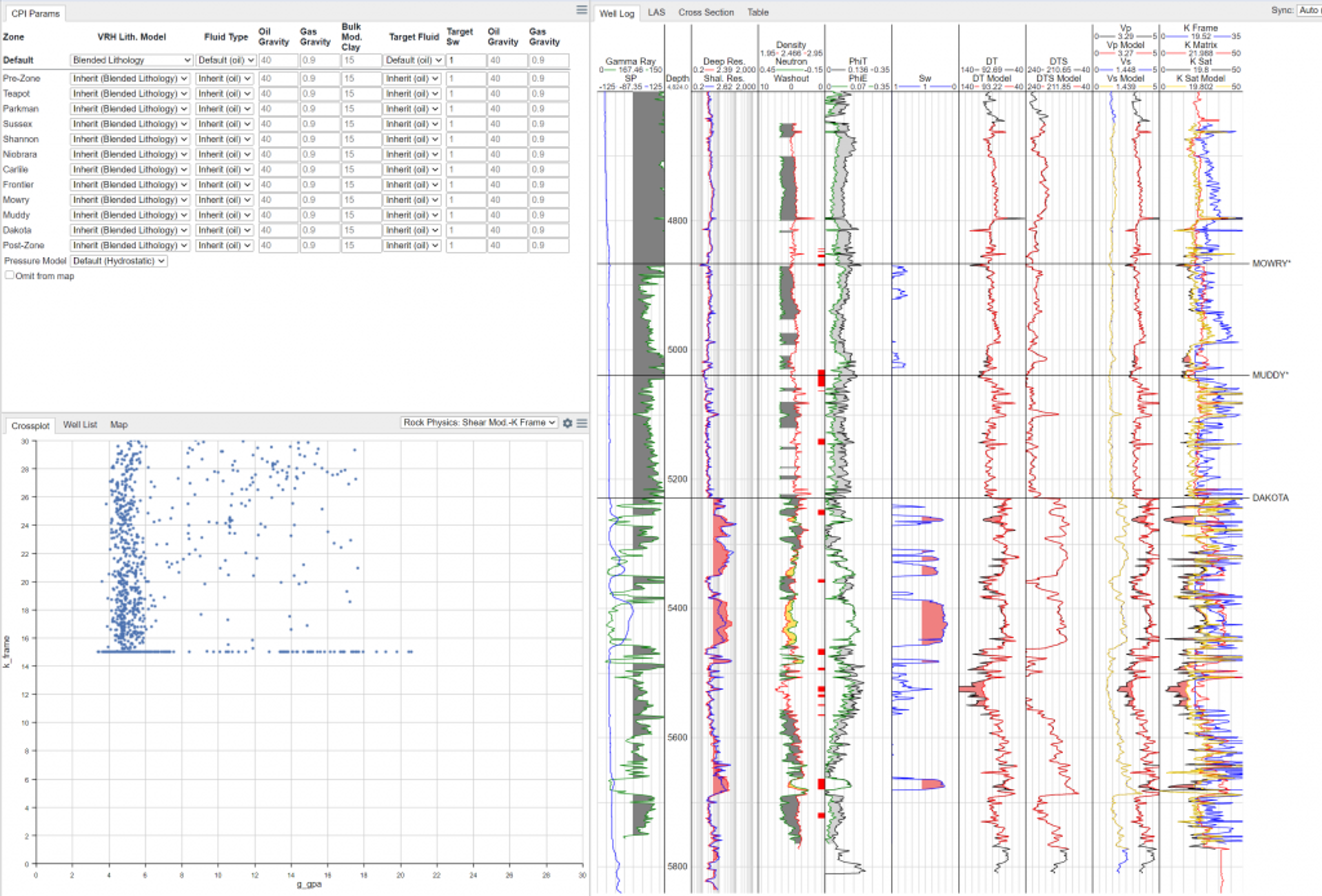
This module is intended to help users evaluate the expected changes in the Vp and Vs responses given the observed hydrocarbon composition and saturation profile and a target hydrocarbon composition and saturation profile. For example, in the screenshot above the sandstone at 5400-5500′ shows good water saturations (< 30%) and modest porosity (~15%) for a conventional sandstone. If an interpreter wanted to understand how the Vp and Vs may be impacted by the presence of brine or a heavier hydrocarbon they could evaluate that impact here.
This type of rock physics workflow is typically done after the bulk of the petrophysical interpretation is done when the interpreter would like to understand if they could expect to use seismic data to differentiate between areas with and without hydrocarbons.
Fluid Substitution Modelling parameters
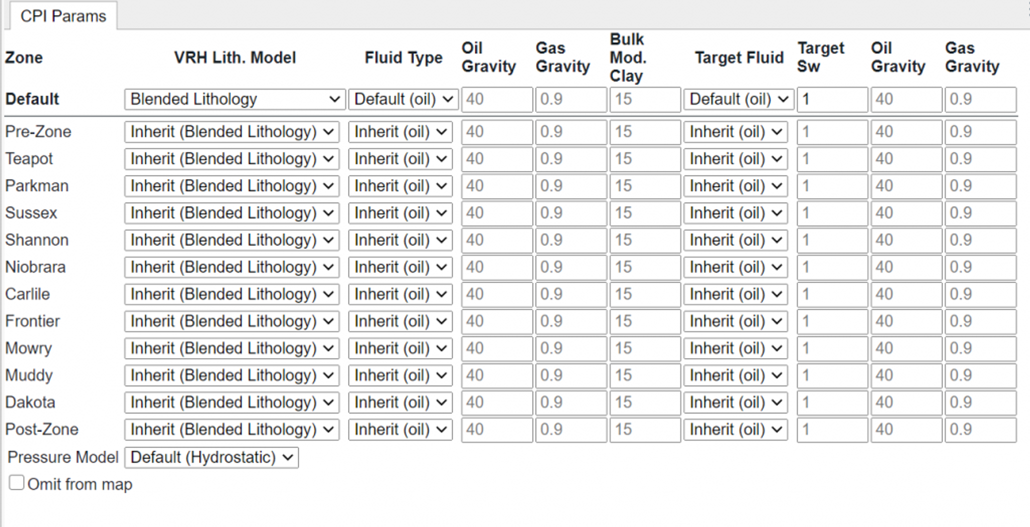
Once the module is activated the user is presented with the following parameters (shown in the screenshot above):
ParameterDescriptionVRH Lithology ModelVoight-Reuss-Hill Lithology Model to be used in calculation of K-matrix modleFluid TypeOil or Gas as the observed fluid type. Used to determine HC fluid parameters shown and correlations used.Oil GravityObserved API gravity of produced oil.Gas GravityObserved API gravity of the produced gas.Bulk Modulus ClayBulk modulus of clay in KPa.Target FluidOil or Gas. Fluid type to model.Target SwWater saturation to use in the model. Set to 1 to model a brine.Oil GravityThe target oil gravity to use in the model.Gas GravityThe target gas gravity to use in the model.Pressure ModelDetermine which pressure model to use in the calculation.
Methodology Details
The module uses the Batzle and Wang methodology for determining the fluid properties for modelling. Key inputs for this are the oil and gas gravity, GOR, temperature, and pressure. The oil and gas gravity are given as inputs. From those, the Vasquez and Beggs correlation is used to determine the GOR. The temperature gradient used in the Water Saturation module is used for the temperature calculation and the user can select between using a hydrostatic pressure or the pressure calculated from Eaton’s sonic or resistivity method via the dropdown menu. Those values are established in the Geomechanics and Pore Pressure module.
The observed response is assumed to occur at the water saturation value determined in the water saturation module. Therefore, it is imperative that this part of the interpretation be completed before moving onto evaluating the effects of changes in saturation.
Also, it is important to note that the method uses the “dts_rphys” curve from the Shear Log Modelling module. Therefore if the well does not have a shear log, it is important that the parameters in this module be carefully evaluated beforehand.
Key Outputs
The table below shows the key outputs from this module
DescriptionMnemonicBulk Modulus of the Frame (K-Frame)k_frameBulk Modulus of the Matrix (K-Matrix)k_matrixSaturated Bulk Modulus (K-Sat)k_sat Model Saturated Bulk Modulus (K-Sat Model) k_sat_modelVp Model vp_modelVs Modelvs_modelDT Modeldt_modelDTS Modeldts_model
Troubleshooting
This is an advanced module that utilizes a number of advanced correlations and methodologies and care must be taken to understand the results. The most common point of frustration is that there is very little difference between the Vp/Vs and DT/DTS model values and the observed values. This is typically because the system is either low porosity (< 15%) and the changes in fluid composition have a minimal effect or that the difference in the observed and modelled values are quite small (e.g., the observed Sw is 35% and the target Sw is 25%). In these cases it might be more useful to evaluate the range of potential model outcomes at extreme end-members such as 100% Sw and the irreducible saturation value.
If the oil gravity parameter(s) are not displaying, check that the fluid type has been set to oil.
If the mineral inversion module has not been utilized it is best to use a VRH Lithology model such as Quartz-Clay or Calcite-Clay which will leverage the clay volumes from the clay volume interpretation module.
Tags
Related Insights
DCA: Type well curves
In this video I demonstrate how to generate a well set filtered by a number of criteria and generate a multi-well type curve. Before starting this video you should already know how to load your data and create a DCA project. If not, please review those videos. Type well curves are generated by creating a decline that represents data from multiple wells.
DCA: Loading Production data
In this video I demonstrate how to load production and well header data for use in a decline curve analysis project. The first step is to gather your data. You’ll need: Production data – this can be in CSV, Excel, or IHS 298 formats. For spreadsheet formats you’ll need columns for API, Date, Oil, Gas, Water (optional), and days of production for that period (optional). Well header data – this can be in CSV, Excel, or IHS 297 formats.
Sample data to get started
Need some sample data to get started? The files below are from data made public by the Wyoming Oil and Gas Commission. These will allow you to get started with petrophysics, mapping, and decline curve analysis. Well header data Formation tops data Deviation survey data Well log data (las files) Production data (csv) or (excel) Wyoming counties shapefile and projection Wyoming townships shapefile and projection Haven’t found the help guide that you are looking for?