Maps and Cross-Sections

Danomics Petrophysics Insights offers mapping and cross-sections to users. Maps are available in both CPI files and Map Files and cross-sections are available in CPI files.

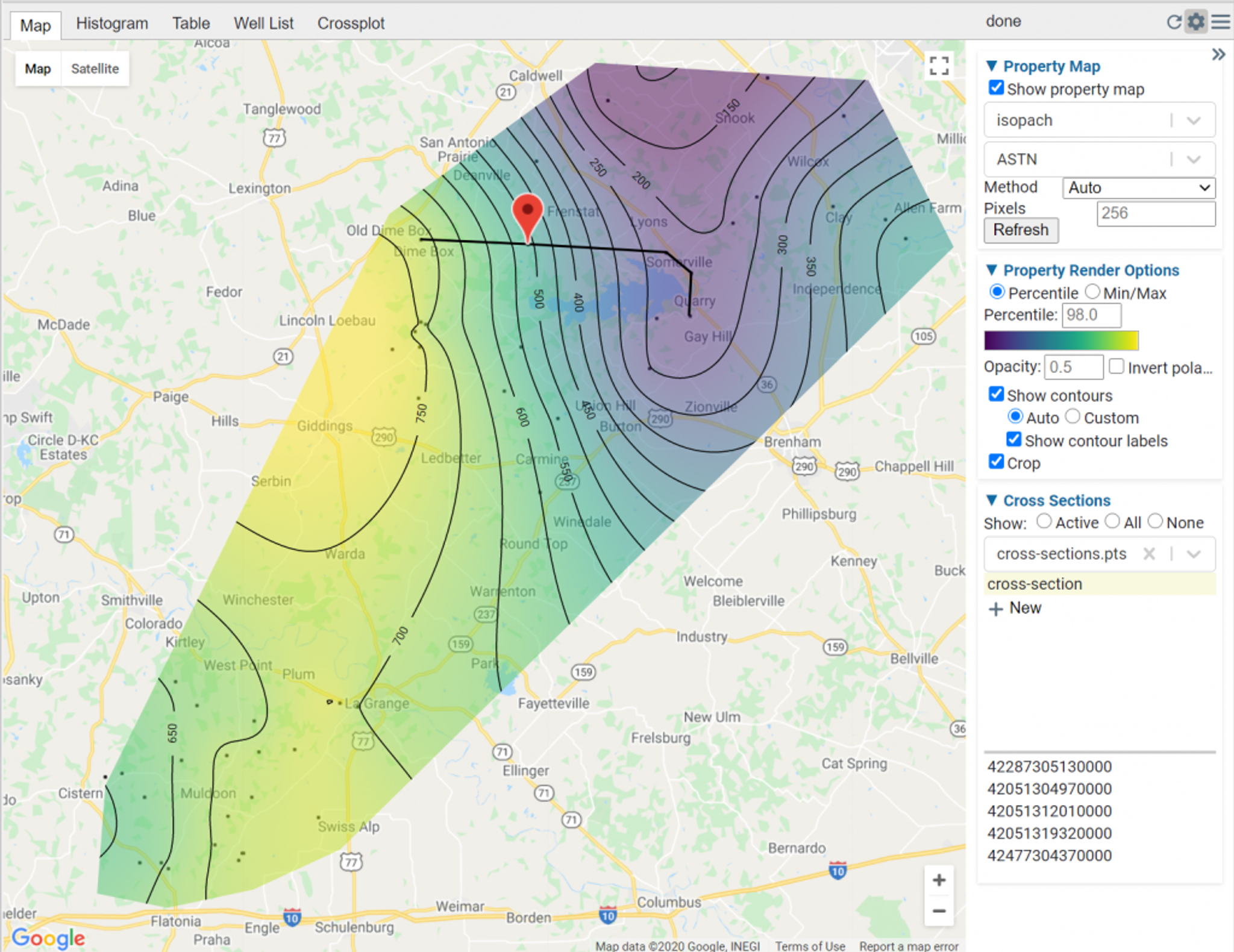
Maps

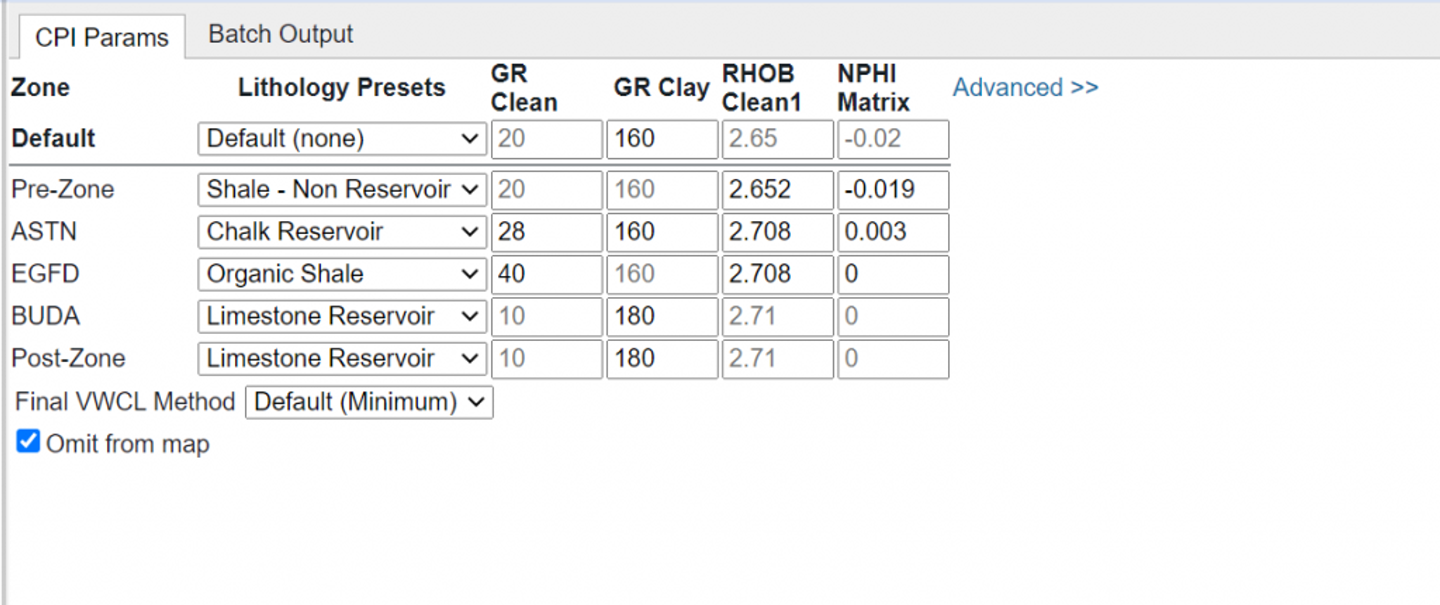
Maps can be displayed in both the CPI and Maps file types. Richer maps with production bubble overlays and shape file overlays can be displayed in the Map file type, while the CPI file type allows users a quick way to evaluate results, albeit with more limited options on displays. Our recommendation is to the CPI file maps while doing interpretations and then use the Map file types to build up presentation ready displays.

Maps are made on a zone-by-zone and property by property basis, with all maps being created for all zones, which allows users to quickly QC multiple zones and properties . Several maps are included in the default set-up and users can extend the set of maps generated by utilizing the CPI Config.

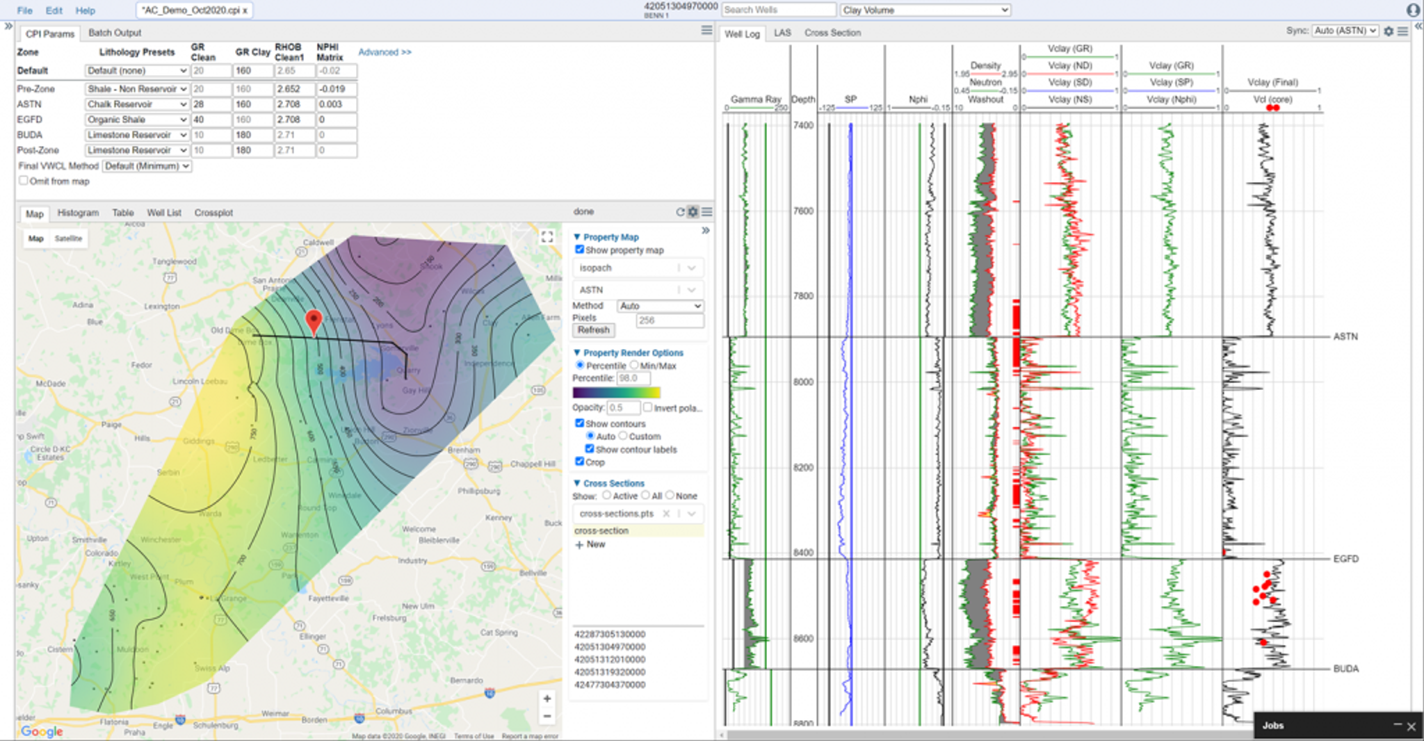
To get started with maps, got to a “Map” tab (if you don’t see this type of tab, click on the three horizontal bars in any window, and select “Add tab >> Map”). Then click the “gear” icon in the top right of the map window to open its settings. Select to show the property map, select the property and zone, and then the maps will be calculated and displayed. You can then quickly use the display options to change the color scales, color ranges, and control contours.

Once you select a zone and property, maps will be generated for all properties for all zones. This generally takes 30 seconds per 100 wells and the status will be tracked in the Jobs queue. Note that for larger mapping jobs the calculation activates a new virtual machine, which will run your map creation. The first time this is done, the virtualization process can take a few minutes to initialize, with subsequent runs being faster.

You can continue working while the map generates in the background as the process is ran in parallel in the cloud. One the maps are generated the selected one will appear in the map area.

At present all gridding, contouring, and color scales are done automatically using program defaults as these maps are intended to assist in the QC process and not for final displays. Maps are automatically clipped to the extent of the data for that property. Therefore, you will likely see a larger map area with more detail for low-level properties like isopach maps and Vclay averages than for high-level maps like OOIP.

The following maps are generated by default:

• structure maps – TVD maps based on well tops

• surface elevation – Map based on imported KB elevation

• zone top – Map based off formation top

• zone base – Map based off formation base

• isopach – Zone thickness as based on well tops. Performed on a “next-top” basis.

• avg_gr_final – Average GR value by formation.

• avg_rhob_final – Average RhoB value by formation.

• avg_nphi_final – Average Nphi value by formation.

• avg_pe_final – Average PE value by formation.

• avg_dt_final – Average DT value by formation.

• avg_resd_final – Average ResD value by formation.

• badhole_summary – Thickness of badhole by formation.

• avg_vwcl – Average Vclay value by formation.

• avg_toc – Average TOC value by formation.

• avg_grain_density – Average Grain Density from the inversion value by formation.

• avg_phit – Average Total Porosity value by formation.

• avg_phie – Average Effective Porosity value by formation.

• avg_sw – Average Water Saturation value by formation.

• gross_res_summary – Thickness of Gross Reservoir within a zone

• net_res_summary – Thickness of Net Reservoir within a zone

• net_pay_summary – Thickness of Net Pay within a zone

• phit_net_res – Average Total Porosity within intervals flagged as Net Res

• phie_net_res – Average Effective Porosity within intervals flagged as Net Res

• sw_net_res – Average Water Saturation within intervals flagged as Net Res

• vwcl_net_pay – Average Vclay within intervals flagged as Net Pay

• phit_net_pay – Average Total Porosity within intervals flagged as Net Pay

• phie_net_pay – Average Effective Porosity within intervals flagged as Net Pay

• sw_net_pay – Average Water Saturation within intervals flagged as Net Pay

• hcpv_summary – Hydrocarbon Pore Volume (PhiE*H*[1-Sw])

• phih_summary – Porosity Thickness (PhiE *H)

• ooip – Original Oil In Place per unit area (see Volumetric Analysis plot)

• ogip – Original Gas in Place per unit area (see Volumetric Analysis plot)

• max_cont_net_res – Thickness of the maximum continuous Net Reservoir Interval

• max_cont_net_pay – Thickness of the maximum continuous Net Pay Interval

• frac_package_summary – Thickness of the maximum continuous Interval from Reservoir Continuity Analysis Module for Net Pay only

• gr_norm_rms – Root mean squared of normalization of GR between key well and non-key well

• sp_norm_rms – Root mean squared of normalization of SP between key well and non-key well

• resd_norm_rms – Root mean squared of normalization of Res Deep between key well and non-key well

• nphi_norm_rms – Root mean squared of normalization of Nphi between key well and non-key well

• rhob_norm_rms – Root mean squared of normalization of RhoB between key well and non-key well

• dt_norm_rms – Root mean squared of normalization of DT between key well and non-key well

The list of maps can be extended via the CPI Config. If you need help doing this, please contact us at support@danomics.com.

To avoid having the maps refresh while working, they remain static until (1) the user hits the refresh button, (2) the user changes the map they want to display, or (3) the user closes and re-opens a project.

If a “problem” well cannot be fixed via overrides to parameters (for example due to bad or missing data) you can omit the well from the map via a single button click. This does not delete the well or its data, but simply excludes it from the mapping.

Cross-Sections

To show a geological cross-section simply click on the Cross Section tab at the bottom of the well log display panel. This will automatically generate a cross-section as shown below:

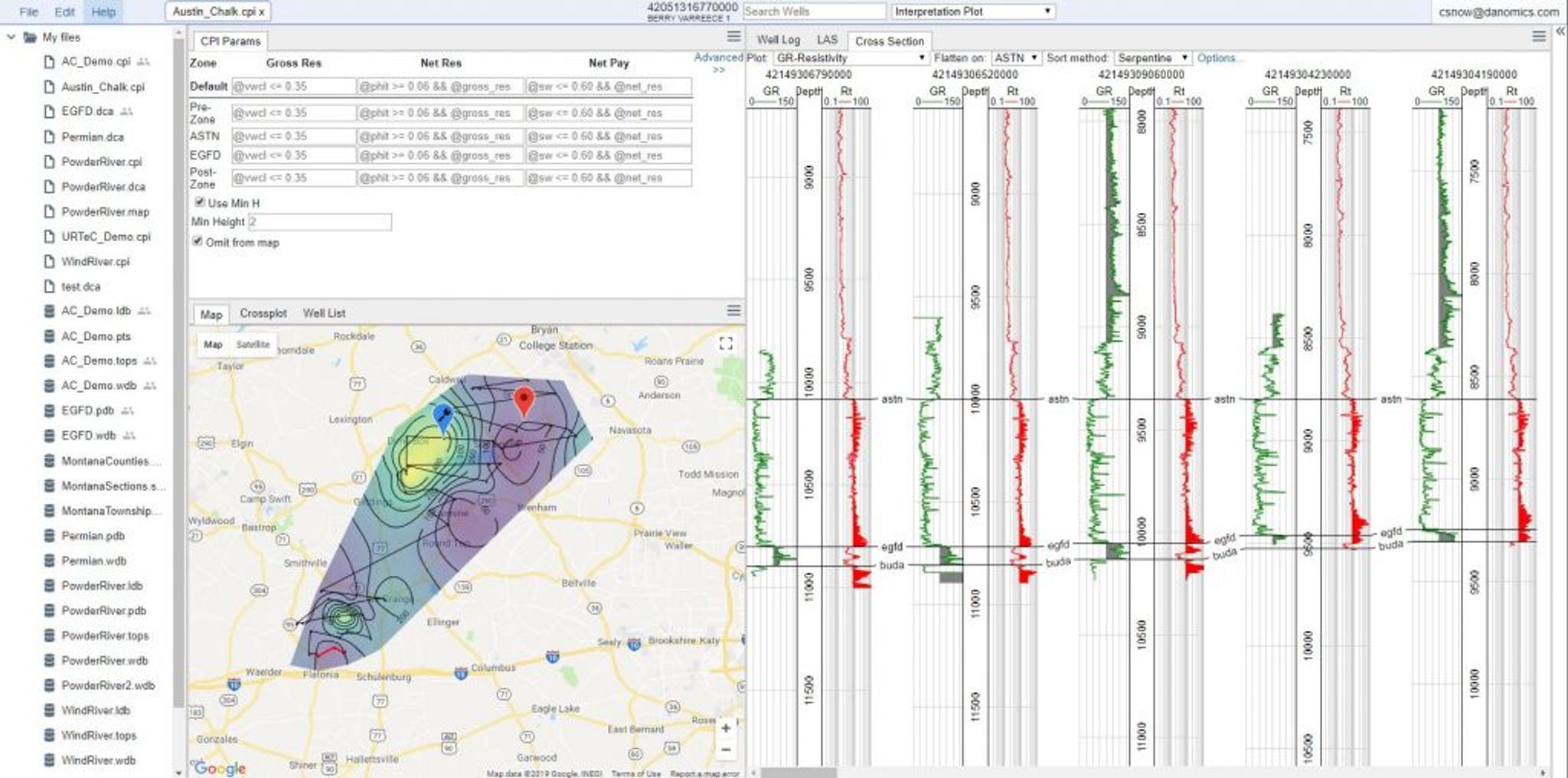
All wells are automatically selected and ordered by default. The cross-section line will appear on the map and the segment shown in the cross-section panel will be highlighted in red. You can jump to a well in the cross-section by clicking it in the map, which makes the cross-section tool useful for QC’ing suspected problem wells. For automatically generated cross-sections the user has options for how to order the wells. There are three methods for ordering the wells, and the “Serpentine” method has options for setting the orientation and the “buffer” for how to assign wells to a segment of the line. This is best visualized by clicking on options and selecting “Show track boxes”.

User-specified cross-sections can also be made within a CPI file. To do so, go to the Map tab, expand the cross-section options area, and in the dropdown menu either click “Create New” or select an existing cross-section database. Cross-sections of this sort are stored in a points database and can be used across multiple projects. To add wells, either right-click on the map and select to add well or right-click and select “Capture to <your-xsection-name> and click well to well.

Wells can be re-ordered by dragging and dropping them in the X-section well list and can be removed by clicking the “x” beside the API number in the cross-section well lsit.

Tops can be modified by dragging and dropping. To select the same top in multiple wells, right click and select the “Capture” option, which will allow you to pick tops from well to well. To turn off, right click and click “Cancel Capture”.

Hints & Tips

Cross-sections can be shown in structural or stratigraphic views. Just choose the “Flatten on:” method you want using the dropdown menu at the top of the cross-section window.

There is an option to map zones based on data coverage. In the “Interpretation” module in the “Advanced” options, you can choose to Map Partial Zones. If selected, zones that are missing data will still be mapped. If not checked, zones with missing data (null values) will not be utilized in the mapping.