Propagating Interpretations
Danomics’ Petrophysics Insights attempts to propagate interpretations from a key well to other wells in a project. Some parameters are propagated as constant values while other parameters undergo a re-mapping process to handle variability that arises due to changes in the subsurface and tool responses.
Parameter Propagation
Some parameter values experience little to no change between wells and can be directly transferred from a key well to other wells in a project, while other parameters can change substantially and need to be varied well-to-well. This can be done via parameter interpolation from spatial tables or grids or by parameter re-mapping.
Users can determine which parameters are spatially varied and which are not. Parameters can be varied well by well using the following options:
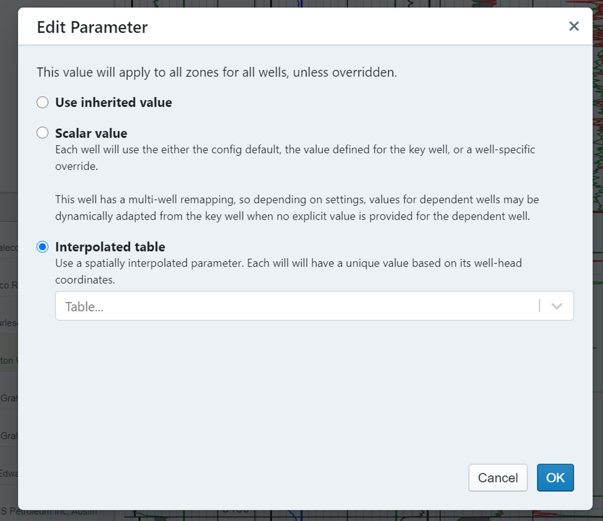
- Interpolation from a spatial table. By clicking on the “gear” icon that is visible when hovering over a parameter box you can access the parameters settings and choose to use a spatial table. This dialog is shown below. A spatial table can either be built from scratch (essentially by manually evaluating a limited number of wells or via importing a series of points. This is often done by doing some calculation in the software, exporting to excel, and then re-importing a modified version.
- Interpolation from a grid file. This is also accessed by clicking on the “gear” icon that is visible when hovering over a parameter box. Once again choose “Interpolated table”, but this time select to use an internally generated gridfile (*.grid).
- Parameter remapping. In the curve normalization module, select the “auto-eval” option for the curves you wish to use for parameter remapping. E.g., “GR auto-eval” will allow parameter re-mapping of the GR_clean and GR_clay endpoints.
Parameter Re-mapping Example
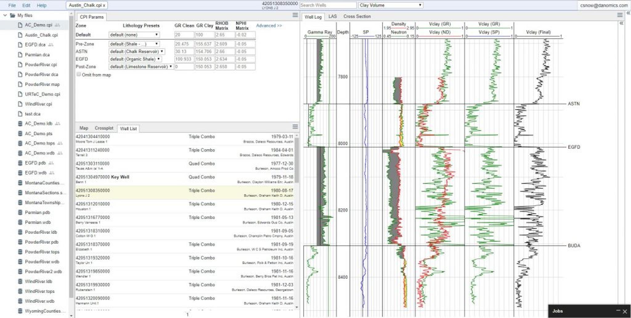
In the example above the key well value for the GR clean parameter was set at 28 in the key well’s ASTN zone and the GR clay was set at 160. Notice that due to the re-mapping algorithms the GR clean in this well has been set at 30, while the GR clay has been set at 155.
This is because the GR curve has a narrower distribution – the low values are a little higher while the high values are a little lower. This re-mapping allows every well to receive its own custom interpretation.
Overrides on non-key wells
Changes from key wells are propagated to all non-key wells. However, values propagated outward can be manually overridden on a well-by-well and zone by zone basis.
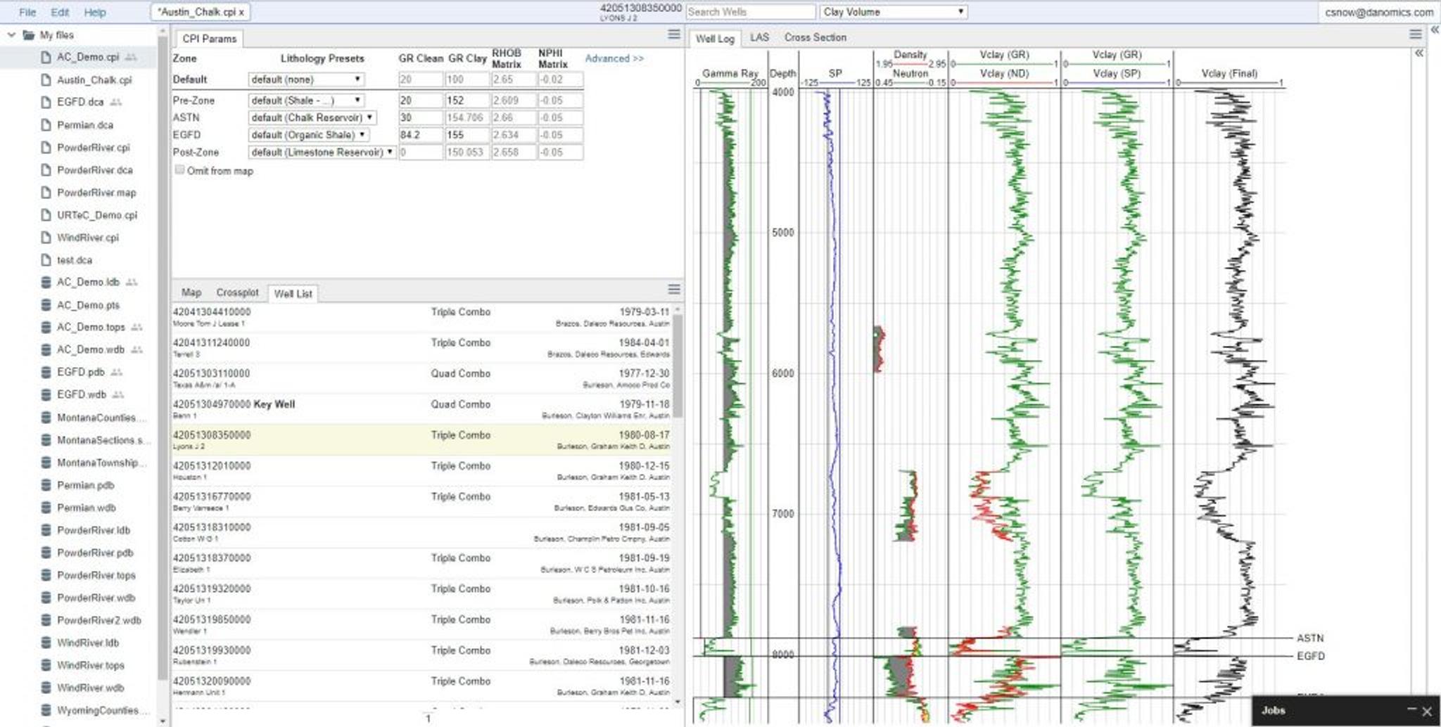
For example, in the screenshot below a number of parameters have been manually changed. For value boxes these are signified by the text showing as black instead of grey, and for methods the dropdown is no longer listed as “default”.
Order of Priority on Parameters
The order of precedence for parameters, in descending order is:
- Formation value manually entered/selected
- Default value manually entered/selected
- Lithology preset manually selected
- Key-well formation value, remapped
- Key-well default value, remapped
- Key-well lithology preset, remapped
- CPI Config default value, remapped
- Built-in parameters (only applies to Depth Step at present)
This means that values typed/selected directly on a zone basis are given the highest priority, followed by default values manually entered for a well. In the absence of a manual entry, remapped/propagated parameters are given priority over CPI Config default values.
Tags
Related Insights
DCA: Type well curves
In this video I demonstrate how to generate a well set filtered by a number of criteria and generate a multi-well type curve. Before starting this video you should already know how to load your data and create a DCA project. If not, please review those videos. Type well curves are generated by creating a decline that represents data from multiple wells.
DCA: Loading Production data
In this video I demonstrate how to load production and well header data for use in a decline curve analysis project. The first step is to gather your data. You’ll need: Production data – this can be in CSV, Excel, or IHS 298 formats. For spreadsheet formats you’ll need columns for API, Date, Oil, Gas, Water (optional), and days of production for that period (optional). Well header data – this can be in CSV, Excel, or IHS 297 formats.
Sample data to get started
Need some sample data to get started? The files below are from data made public by the Wyoming Oil and Gas Commission. These will allow you to get started with petrophysics, mapping, and decline curve analysis. Well header data Formation tops data Deviation survey data Well log data (las files) Production data (csv) or (excel) Wyoming counties shapefile and projection Wyoming townships shapefile and projection Haven’t found the help guide that you are looking for?