Pore Pressure

Note: This module originally included many geomechanics options. These have been moved to the Geomechanics and 1D Geomechanical Earth Model tabs to keep make each of the modules more focused.

In Danomics Petrophysics Insights users are guided through a workflow that walks them through a number of modules. These modules are located via a dropdown menu at the top center of the window. The modules are listed in the order in which a user should ideally proceed through a project. However, this order is not strictly enforced and the user can start at any module and can seamlessly move both forward and back through the modules. This help article will focus on the Pore Pressure module.

Pore Pressure

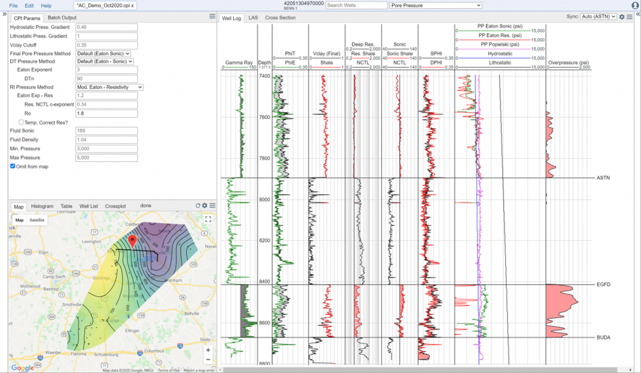
To activate the Pore Pressure & Geomechanics module, select “Pore Pressure” from the module dropdown selection menu located in the top-middle area of the page. This module allows for calculation of pore-pressure via the Eaton Sonic, Eaton Resistivity, Modified Eaton Sonic, Modified Eaton Resistivity, and Popielski methodologies.

Method Parameters and Criteria

The user has options for entering the hydrostatic and lithostatic pressure gradients. Lithostatic will preferably be calculated from the density curve if available. These two curves are useful calibration points and are displayed in the pressure track.

The Vclay Cutoff parameter allows the user to set what is considered “clay” for the purposes of the Eaton methods, which only calculate pore pressure in clay-rich intervals. Everything greater than or equal to the value will be used for calculations and will be highlighted in red on the Vclay track.

The Final Pore Pressure Method allows the user to select which results will be used when calculating overpressure and when moving into the Geomechanics and 1D Geomechanical Earth Model modules.

The parameters for the Eaton and Modified Eat methods are available for each method. For the Popielski method the user will need to select a fluid value for the Sonic and Density, and a Min/Max pressure to calibrate the method.

The results are all shown on the second track from the right along with the hydrostatic and lithostatic pressures. The Overpressure curve is a composite of the hydrostatic pressure gradient and the overpressure from the final pore pressure method, if present.

Key Outputs

The following are the key outputs from this module:

Output CurveDescriptionpp_eaton_dtPore pressure from the Eaton or Modified Eaton Sonicpp_eaton_res Pore pressure from the Eaton or Modified Eaton Resistivitypp_popielski Pore pressure from the Popielski methodpore_pressure_finalFinal Pore Pressure from selected methodologyoverpressureDifference of Final Pore Pressure and Hydrostatic pressurehydrostaticHydrostatic pressure.overburdenLithostatic pressure

Tips and Tricks

• When evaluating pore pressure it is important to ensure that you are able to match the hydrostatic pressure in zones that are not suspected to be overpressured. This is a valuable anchor point.
• The Eaton methods should only be applied to shales. The Eaton resistivity method almost always underestimates pressures in organic shales because of the excess resistivity due to hydrocarbon presence.
• The Popielski method requires anchoring on a maximum and minimum value within the stats window. These should be set carefully.